Fsolve matlab система нелинейных уравнений

Решение систем нелинейных уравнений в Matlab

Доброго времени суток! В этой статье мы поговорим о решении систем нелинейных алгебраических уравнений в Matlab. Вслед за решением нелинейных уравнений, переходим к их системам, рассмотрим несколько методов реализации в Matlab.

Общая информация

Итак, в прошлой статье мы рассмотрели нелинейные уравнения и теперь необходимо решить системы таких уравнений. Система представляет собой набор нелинейных уравнений (их может быть два или более), для которых иногда возможно найти решение, которое будет подходить ко всем уравнениям в системе.

В стандартном виде, количество неизвестных переменных равно количеству уравнений в системе. Необходимо найти набор неизвестных переменных, которые при подставлении в уравнения будут приближать значение уравнения к 0. Иногда таких наборов может быть несколько, даже бесконечно много, а иногда решений не существует.

Чтобы решить СНАУ, необходимо воспользоваться итеративными методами. Это методы, которые за определенное количество шагов получают решение с определенной точностью. Также очень важно при решении задать достаточно близкое начальное приближение, то есть такой набор переменных, которые близки к решению. Если решается система из 2 уравнений, то приближение находится с помощью построение графика двух функций.

Далее, мы рассмотрим стандартный оператор Matlab для решения систем нелинейных алгебраических уравнений, а также напишем метод простых итераций и метод Ньютона.

Оператор Matlab для решения СНАУ

В среде Matlab существует оператор fsolve, который позволяет решить систему нелинейных уравнений. Сразу рассмотрим задачу, которую, забегая вперед, решим и другими методами для проверки.

Решить систему нелинейных уравнений с точность 10 -2 :
cos(x-1) + y = 0.5
x-cos(y) = 3

Нам дана система из 2 нелинейных уравнений и сначала лучше всего построить график. Воспользуемся командой ezplot в Matlab, только не забудем преобразовать уравнения к стандартному виду, где правая часть равна 0:

Функция ezplot строит график, принимая символьную запись уравнения, а для задания цвета и толщины линии воспользуемся функцией set. Посмотрим на вывод:

Как видно из графика, есть одно пересечение функций — то есть одно единственное решение данной системы нелинейных уравнений. И, как было сказано, по графику найдем приближение. Возьмем его как (3.0, 1.0). Теперь найдем решение с его помощью:

Создадим функцию m-файлом fun.m и поместим туда следующий код:

Заметьте, что эта функция принимает вектор приближений и возвращает вектор значений функции. То есть, вместо x здесь x(1), а вместо y — x(2). Это необходимо, потому что fsolve работает с векторами, а не с отдельными переменными.

И наконец, допишем функцию fsolve к коду построения графика таким образом:

Таким образом у нас образуется два m-файла. Первый строит график и вызывает функцию fsolve, а второй необходим для расчета самих значений функций. Если вы что-то не поняли, то в конце статьи будут исходники.

И в конце, приведем результаты:

xr (это вектор решений) =
3.3559 1.2069

fr (это значения функций при таких xr, они должны быть близки к 0) =
1.0e-09 *
0.5420 0.6829

ex (параметр сходимости, если он равен 1, то все сошлось) =
1

И, как же без графика с ответом:

Метод простых итераций в Matlab для решения СНАУ

Теперь переходим к методам, которые запрограммируем сами. Первый из них — метод простых итераций. Он заключается в том, что итеративно приближается к решению, конечно же, с заданной точностью. Алгоритм метода достаточно прост:

1. Если возможно, строим график.
2. Из каждого уравнения выражаем неизвестную переменную след. образом: из 1 уравнения выражаем x1, из второго — x2, и т.д.
3. Выбираем начальное приближение X0, например (3.0 1.0)
4. Рассчитываем значение x1, x2. xn, которые получили на шаге 2, подставив значения из приближения X0.
5. Проверяем условие сходимости, (X-X0) должно быть меньше точности
6. Если 5 пункт не выполнился, то повторяем 4 пункт.

И перейдем к практике, тут станет все понятнее.
Решить систему нелинейных уравнений методом простых итераций с точность 10 -2 :
cos(x-1) + y = 0.5
x-cos(y) = 3

График мы уже строили в предыдущем пункте, поэтому переходим к преобразованию. Увидим, что x из первого уравнения выразить сложно, поэтому поменяем местами уравнения, это не повлияет на решение:

x-cos(y) = 3
cos(x-1) + y = 0.5

Далее приведем код в Matlab:

В этой части мы выразили x1 и x2 (у нас это ‘x’ и ‘y’) и задали точность.

В этой части в цикле выполняются пункты 4-6. То есть итеративно меняются значения x и y, пока отличия от предыдущего значения не станет меньше заданной точности.

k = 10
x = 3.3587
y = 1.2088

Как видно, результаты немного отличаются от предыдущего пункта. Это связано с заданной точностью, можете попробовать поменять точность и увидите, что результаты станут такими же, как и при решении стандартным методом Matlab.

Метод Ньютона в Matlab для решения СНАУ

Решение систем нелинейных уравнений в Matlab методом Ньютона является более эффективным, чем использование метода простых итераций. Сразу же представим алгоритм, а затем перейдем к реализации.

1. Если возможно, строим график.
2. Выбираем начальное приближение X0, например (3.0 1.0)
3. Рассчитываем матрицу Якоби w, это матрица частных производных каждого уравнения, считаем ее определитель для X0.
4. Находим вектор приращений, который рассчитывается как dx = -w -1 * f(X0)
5. Находим вектор решения X = X0 + dx
6. Проверяем условие сходимости, (X-X0) должно быть меньше точности

Далее, решим тот же пример, что и в предыдущих пунктах. Его график мы уже строили и начальное приближение останется таким же.
Решить систему нелинейных уравнений методом Ньютона с точность 10 -2 :
cos(x-1) + y = 0.5
x-cos(y) = 3

Перейдем к коду:

Сначала зададим начальное приближение. Затем необходимо просчитать матрицу Якоби, то есть частные производные по всем переменным. Воспользуемся символьным дифференцированием в Matlab, а именно командой diff с использованием символьных переменных.

Далее, сделаем первую итерацию метода, чтобы получить вектор выходных значений X, а потом уже сравнивать его с приближением в цикле.

В этой части кода выполняем первую итерацию, чтобы получить вектор решения и сравнивать его с вектором начального приближения. Отметим, чтобы посчитать значение символьной функции в Matlab, необходимо воспользоваться функцией subs. Эта функция заменяет переменную на числовое значение. Затем функция double рассчитает это числовое значение.

Все действия, которые были выполнены для расчета производных, на самом деле можно было не производить, а сразу же задать производные. Именно так мы и поступим в цикле.

В этой части кода выполняется цикл по расчету решения с заданной точностью. Еще раз отметим, что если в первой итерации до цикла были использованы функции diff, double и subs для вычисления производной в Matlab, то в самом цикле матрица якоби была явно задана этими частными производными. Это сделано, чтобы показать возможности среды Matlab.

За 3 итерации достигнут правильный результат. Также важно сказать, что иногда такие методы могут зацикливаться и не закончить расчеты. Чтобы такого не было, мы прописали проверку на количество итераций и запретили выполнение более 100 итераций.

Заключение

В этой статье мы познакомились с основными понятиями систем нелинейных алгебраических уравнений в Matlab. Рассмотрели несколько вариантов их решения, как стандартными операторами Matlab, так и запрограммированными методами простых итераций и Ньютона.

fsolve

Solve system of nonlinear equations

Syntax

Description

Nonlinear system solver

Solves a problem specified by

for x, where F( x) is a function that returns a vector value.

x is a vector or a matrix; see Matrix Arguments.

x = fsolve( fun , x0 ) starts at x0 and tries to solve the equations fun(x) = 0, an array of zeros.

Note

Passing Extra Parameters explains how to pass extra parameters to the vector function fun(x) , if necessary. See Solve Parameterized Equation.

x = fsolve( fun , x0 , options ) solves the equations with the optimization options specified in options . Use optimoptions to set these options.

x = fsolve( problem ) solves problem , a structure described in problem .

[ x , fval ] = fsolve( ___ ) , for any syntax, returns the value of the objective function fun at the solution x .

[ x , fval , exitflag , output ] = fsolve( ___ ) additionally returns a value exitflag that describes the exit condition of fsolve , and a structure output with information about the optimization process.

[ x , fval , exitflag , output , jacobian ] = fsolve( ___ ) returns the Jacobian of fun at the solution x .

Examples

Solution of 2-D Nonlinear System

This example shows how to solve two nonlinear equations in two variables. The equations are

Convert the equations to the form .

Write a function that computes the left-hand side of these two equations.

Save this code as a file named root2d.m on your MATLAB® path.

Solve the system of equations starting at the point [0,0] .

Solution with Nondefault Options

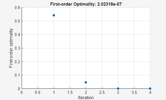
Examine the solution process for a nonlinear system.

Set options to have no display and a plot function that displays the first-order optimality, which should converge to 0 as the algorithm iterates.

The equations in the nonlinear system are

Convert the equations to the form .

Write a function that computes the left-hand side of these two equations.

Save this code as a file named root2d.m on your MATLAB® path.

Solve the nonlinear system starting from the point [0,0] and observe the solution process.

Solve Parameterized Equation

You can parameterize equations as described in the topic Passing Extra Parameters. For example, the paramfun helper function at the end of this example creates the following equation system parameterized by c :

2 x 1 + x 2 = exp ( c x 1 ) — x 1 + 2 x 2 = exp ( c x 2 ) .

To solve the system for a particular value, in this case c = — 1 , set c in the workspace and create an anonymous function in x from paramfun .

Solve the system starting from the point x0 = [0 1] .

To solve for a different value of c , enter c in the workspace and create the fun function again, so it has the new c value.

This code creates the paramfun helper function.

Solve a Problem Structure

Create a problem structure for fsolve and solve the problem.

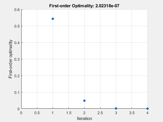
Solve the same problem as in Solution with Nondefault Options, but formulate the problem using a problem structure.

Set options for the problem to have no display and a plot function that displays the first-order optimality, which should converge to 0 as the algorithm iterates.

The equations in the nonlinear system are

Convert the equations to the form .

Write a function that computes the left-hand side of these two equations.

Save this code as a file named root2d.m on your MATLAB® path.

Create the remaining fields in the problem structure.

Solve the problem.

Solution Process of Nonlinear System

This example returns the iterative display showing the solution process for the system of two equations and two unknowns

2 x 1 — x 2 = e — x 1 — x 1 + 2 x 2 = e — x 2 .

Rewrite the equations in the form F ( x ) = 0 :

2 x 1 — x 2 — e — x 1 = 0 — x 1 + 2 x 2 — e — x 2 = 0 .

Start your search for a solution at x0 = [-5 -5] .

First, write a function that computes F , the values of the equations at x .

Create the initial point x0 .

Set options to return iterative display.

Solve the equations.

The iterative display shows f(x) , which is the square of the norm of the function F(x) . This value decreases to near zero as the iterations proceed. The first-order optimality measure likewise decreases to near zero as the iterations proceed. These entries show the convergence of the iterations to a solution. For the meanings of the other entries, see Iterative Display.

The fval output gives the function value F(x) , which should be zero at a solution (to within the FunctionTolerance tolerance).

Examine Matrix Equation Solution

Find a matrix X that satisfies

X * X * X = [ 1 2 3 4 ] ,

starting at the point x0 = [1,1;1,1] . Create an anonymous function that calculates the matrix equation and create the point x0 .

Set options to have no display.

Examine the fsolve outputs to see the solution quality and process.

The exit flag value 1 indicates that the solution is reliable. To verify this manually, calculate the residual (sum of squares of fval) to see how close it is to zero.

This small residual confirms that x is a solution.

You can see in the output structure how many iterations and function evaluations fsolve performed to find the solution.

Input Arguments

fun — Nonlinear equations to solve
function handle | function name

Nonlinear equations to solve, specified as a function handle or function name. fun is a function that accepts a vector x and returns a vector F , the nonlinear equations evaluated at x . The equations to solve are F = 0 for all components of F . The function fun can be specified as a function handle for a file

where myfun is a MATLAB ® function such as

fun can also be a function handle for an anonymous function.

fsolve passes x to your objective function in the shape of the x0 argument. For example, if x0 is a 5-by-3 array, then fsolve passes x to fun as a 5-by-3 array.

If the Jacobian can also be computed and the ‘SpecifyObjectiveGradient’ option is true , set by

the function fun must return, in a second output argument, the Jacobian value J , a matrix, at x .

If fun returns a vector (matrix) of m components and x has length n , where n is the length of x0 , the Jacobian J is an m -by- n matrix where J(i,j) is the partial derivative of F(i) with respect to x(j) . (The Jacobian J is the transpose of the gradient of F .)

Example: fun = @(x)x*x*x-[1,2;3,4]

Data Types: char | function_handle | string

x0 — Initial point
real vector | real array

Initial point, specified as a real vector or real array. fsolve uses the number of elements in and size of x0 to determine the number and size of variables that fun accepts.

Example: x0 = [1,2,3,4]

Data Types: double

options — Optimization options
output of optimoptions | structure as optimset returns

Optimization options, specified as the output of optimoptions or a structure such as optimset returns.

Some options apply to all algorithms, and others are relevant for particular algorithms. See Optimization Options Reference for detailed information.

Some options are absent from the optimoptions display. These options appear in italics in the following table. For details, see View Options.

Choose between ‘trust-region-dogleg’ (default), ‘trust-region’ , and ‘levenberg-marquardt’ .

The Algorithm option specifies a preference for which algorithm to use. It is only a preference because for the trust-region algorithm, the nonlinear system of equations cannot be underdetermined; that is, the number of equations (the number of elements of F returned by fun ) must be at least as many as the length of x . Similarly, for the trust-region-dogleg algorithm, the number of equations must be the same as the length of x . fsolve uses the Levenberg-Marquardt algorithm when the selected algorithm is unavailable. For more information on choosing the algorithm, see Choosing the Algorithm.

To set some algorithm options using optimset instead of optimoptions :

Algorithm — Set the algorithm to ‘trust-region-reflective’ instead of ‘trust-region’ .

InitDamping — Set the initial Levenberg-Marquardt parameter λ by setting Algorithm to a cell array such as <'levenberg-marquardt',.005>.

Display diagnostic information about the function to be minimized or solved. The choices are ‘on’ or the default ‘off’ .

Maximum change in variables for finite-difference gradients (a positive scalar). The default is Inf .

Minimum change in variables for finite-difference gradients (a positive scalar). The default is 0 .

‘off’ or ‘none’ displays no output.

‘iter’ displays output at each iteration, and gives the default exit message.

‘iter-detailed’ displays output at each iteration, and gives the technical exit message.

‘final’ (default) displays just the final output, and gives the default exit message.

‘final-detailed’ displays just the final output, and gives the technical exit message.

Scalar or vector step size factor for finite differences. When you set FiniteDifferenceStepSize to a vector v , the forward finite differences delta are

For optimset , the name is FinDiffRelStep . See Current and Legacy Option Names.

Finite differences, used to estimate gradients, are either ‘forward’ (default), or ‘central’ (centered). ‘central’ takes twice as many function evaluations, but should be more accurate.

The algorithm is careful to obey bounds when estimating both types of finite differences. So, for example, it could take a backward, rather than a forward, difference to avoid evaluating at a point outside bounds.

For optimset , the name is FinDiffType . See Current and Legacy Option Names.

Termination tolerance on the function value, a positive scalar. The default is 1e-6 . See Tolerances and Stopping Criteria.

For optimset , the name is TolFun . See Current and Legacy Option Names.

Check whether objective function values are valid. ‘on’ displays an error when the objective function returns a value that is complex , Inf , or NaN . The default, ‘off’ , displays no error.

Maximum number of function evaluations allowed, a positive integer. The default is 100*numberOfVariables . See Tolerances and Stopping Criteria and Iterations and Function Counts.

For optimset , the name is MaxFunEvals . See Current and Legacy Option Names.

Maximum number of iterations allowed, a positive integer. The default is 400 . See Tolerances and Stopping Criteria and Iterations and Function Counts.

For optimset , the name is MaxIter . See Current and Legacy Option Names.

Termination tolerance on the first-order optimality (a positive scalar). The default is 1e-6 . See First-Order Optimality Measure.

Internally, the ‘levenberg-marquardt’ algorithm uses an optimality tolerance (stopping criterion) of 1e-4 times FunctionTolerance and does not use OptimalityTolerance .

Specify one or more user-defined functions that an optimization function calls at each iteration. Pass a function handle or a cell array of function handles. The default is none ( [] ). See Output Function and Plot Function Syntax.

Plots various measures of progress while the algorithm executes; select from predefined plots or write your own. Pass a built-in plot function name, a function handle, or a cell array of built-in plot function names or function handles. For custom plot functions, pass function handles. The default is none ( [] ):

‘optimplotx’ plots the current point.

‘optimplotfunccount’ plots the function count.

‘optimplotfval’ plots the function value.

‘optimplotstepsize’ plots the step size.

‘optimplotfirstorderopt’ plots the first-order optimality measure.

Custom plot functions use the same syntax as output functions. See Output Functions for Optimization Toolbox™ and Output Function and Plot Function Syntax.

For optimset , the name is PlotFcns . See Current and Legacy Option Names.

If true , fsolve uses a user-defined Jacobian (defined in fun ), or Jacobian information (when using JacobianMultiplyFcn ), for the objective function. If false (default), fsolve approximates the Jacobian using finite differences.

For optimset , the name is Jacobian and the values are ‘on’ or ‘off’ . See Current and Legacy Option Names.

Termination tolerance on x , a positive scalar. The default is 1e-6 . See Tolerances and Stopping Criteria.

For optimset , the name is TolX . See Current and Legacy Option Names.

Typical x values. The number of elements in TypicalX is equal to the number of elements in x0 , the starting point. The default value is ones(numberofvariables,1) . fsolve uses TypicalX for scaling finite differences for gradient estimation.

The trust-region-dogleg algorithm uses TypicalX as the diagonal terms of a scaling matrix.

When true , fsolve estimates gradients in parallel. Disable by setting to the default, false . See Parallel Computing.

Jacobian multiply function, specified as a function handle. For large-scale structured problems, this function computes the Jacobian matrix product J*Y , J’*Y , or J’*(J*Y) without actually forming J . The function is of the form

where Jinfo contains a matrix used to compute J*Y (or J’*Y , or J’*(J*Y) ). The first argument Jinfo must be the same as the second argument returned by the objective function fun , for example, in

Y is a matrix that has the same number of rows as there are dimensions in the problem. flag determines which product to compute:

If flag == 0 , W = J’*(J*Y) .

If flag > 0 , W = J*Y .

In each case, J is not formed explicitly. fsolve uses Jinfo to compute the preconditioner. See Passing Extra Parameters for information on how to supply values for any additional parameters jmfun needs.

Note

‘SpecifyObjectiveGradient’ must be set to true for fsolve to pass Jinfo from fun to jmfun .

For optimset , the name is JacobMult . See Current and Legacy Option Names.

Sparsity pattern of the Jacobian for finite differencing. Set JacobPattern(i,j) = 1 when fun(i) depends on x(j) . Otherwise, set JacobPattern(i,j) = 0 . In other words, JacobPattern(i,j) = 1 when you can have ∂ fun(i) /∂ x(j) ≠ 0.

Use JacobPattern when it is inconvenient to compute the Jacobian matrix J in fun , though you can determine (say, by inspection) when fun(i) depends on x(j) . fsolve can approximate J via sparse finite differences when you give JacobPattern .

In the worst case, if the structure is unknown, do not set JacobPattern . The default behavior is as if JacobPattern is a dense matrix of ones. Then fsolve computes a full finite-difference approximation in each iteration. This can be very expensive for large problems, so it is usually better to determine the sparsity structure.

Maximum number of PCG (preconditioned conjugate gradient) iterations, a positive scalar. The default is max(1,floor(numberOfVariables/2)) . For more information, see Equation Solving Algorithms.

Upper bandwidth of preconditioner for PCG, a nonnegative integer. The default PrecondBandWidth is Inf , which means a direct factorization (Cholesky) is used rather than the conjugate gradients (CG). The direct factorization is computationally more expensive than CG, but produces a better quality step towards the solution. Set PrecondBandWidth to 0 for diagonal preconditioning (upper bandwidth of 0). For some problems, an intermediate bandwidth reduces the number of PCG iterations.

Determines how the iteration step is calculated. The default, ‘factorization’ , takes a slower but more accurate step than ‘cg’ . See Trust-Region Algorithm.

Termination tolerance on the PCG iteration, a positive scalar. The default is 0.1 .

Initial value of the Levenberg-Marquardt parameter, a positive scalar. Default is 1e-2 . For details, see Levenberg-Marquardt Method.

‘jacobian’ can sometimes improve the convergence of a poorly scaled problem. The default is ‘none’ .

Example: options = optimoptions(‘fsolve’,’FiniteDifferenceType’,’central’)

Fsolve matlab система нелинейных уравнений

Solve a system of nonlinear equations

for x, where x is a vector and F(x) is a function that returns a vector value.

fsolve finds a root (zero) of a system of nonlinear equations.

x = fsolve(fun,x0) starts at x0 and tries to solve the equations described in fun .

x = fsolve(fun,x0,options) minimizes with the optimization parameters specified in the structure options . Use optimset to set these parameters.

x = fsolve(fun,x0,options,P1,P2. ) passes the problem-dependent parameters P1 , P2 , etc., directly to the function fun . Pass an empty matrix for options to use the default values for options .

[x,fval] = fsolve(fun,x0) returns the value of the objective function fun at the solution x .

[x,fval,exitflag] = fsolve(. ) returns a value exitflag that describes the exit condition.

[x,fval,exitflag,output] = fsolve(. ) returns a structure output that contains information about the optimization.

[x,fval,exitflag,output,jacobian] = fsolve(. ) returns the Jacobian of fun at the solution x .

Function Arguments contains general descriptions of arguments passed in to fsolve . This section provides function-specific details for fun and options :

Function Arguments contains general descriptions of arguments returned by fsolve . This section provides function-specific details for exitflag and output :

Optimization options parameters used by fsolve . Some parameters apply to all algorithms, some are only relevant when using the large-scale algorithm, and others are only relevant when using the medium-scale algorithm.You can use optimset to set or change the values of these fields in the parameters structure, options . See Optimization Parameters, for detailed information.

We start by describing the LargeScale option since it states a preference for which algorithm to use. It is only a preference since certain conditions must be met to use the large-scale algorithm. For fsolve , the nonlinear system of equations cannot be underdetermined; that is, the number of equations (the number of elements of F returned by fun ) must be at least as many as the length of x or else the medium-scale algorithm is used:

Medium-Scale and Large-Scale Algorithms. These parameters are used by both the medium-scale and large-scale algorithms:

Large-Scale Algorithm Only. These parameters are used only by the large-scale algorithm:

Medium-Scale Algorithm Only. These parameters are used only by the medium-scale algorithm:

Example 1. This example finds a zero of the system of two equations and two unknowns

Thus we want to solve the following system for x

starting at x0 = [-5 -5] .

First, write an M-file that computes F , the values of the equations at x .

Next, call an optimization routine.

After 33 function evaluations, a zero is found.

Example 2. Find a matrix x that satisfies the equation

starting at the point x= [1,1; 1,1] .

First, write an M-file that computes the equations to be solved.

Next, invoke an optimization routine.

The solution is

and the residual is close to zero.

If the system of equations is linear, then use the \ (the backslash operator; see help slash ) for better speed and accuracy. For example, to find the solution to the following linear system of equations.

Then the problem is formulated and solved as

The Gauss-Newton, Levenberg-Marquardt, and large-scale methods are based on the nonlinear least-squares algorithms also used in lsqnonlin . Use one of these methods if the system may not have a zero. The algorithm still returns a point where the residual is small. However, if the Jacobian of the system is singular, the algorithm may converge to a point that is not a solution of the system of equations (see Limitations and Diagnostics below).

Large-Scale Optimization. fsolve , with the LargeScale parameter set to ‘on’ with optimset , uses the large-scale algorithm if possible. This algorithm is a subspace trust region method and is based on the interior-reflective Newton method described in [1],[2]. Each iteration involves the approximate solution of a large linear system using the method of preconditioned conjugate gradients (PCG). See Trust-Region Methods for Nonlinear Minimization, and Preconditioned Conjugate Gradients.

Medium-Scale Optimization. b y default fsolve chooses the medium-scale algorithm and uses the trust-region dogleg method. The algorithm is a variant of the Powell dogleg method described in [8]. It is similar in nature to the algorithm implemented in [7].

Alternatively, you can select a Gauss-Newton method [3] with line-search, or a Levenberg-Marquardt method [4], [5], [6] with line-search. The choice of algorithm is made by setting the NonlEqnAlgorithm parameter to ‘dogleg’ (default), ‘lm’ , or ‘gn’ .

The default line search algorithm for the Levenberg-Marquardt and Gauss-Newton methods, i.e., the LineSearchType parameter set to ‘quadcubic’ , is a safeguarded mixed quadratic and cubic polynomial interpolation and extrapolation method. A safeguarded cubic polynomial method can be selected by setting LineSearchType to ‘cubicpoly’ . This method generally requires fewer function evaluations but more gradient evaluations. Thus, if gradients are being supplied and can be calculated inexpensively, the cubic polynomial line search method is preferable. The algorithms used are described fully in the Standard Algorithms chapter.

Medium and Large Scale Optimization. fsolve may converge to a nonzero point and give this message

In this case, run fsolve again with other starting values.

Medium Scale Optimization. For the trust-region dogleg method, fsolve stops if the step size becomes to small and it can make no more progress. fsolve gives this message

In this case, run fsolve again with other starting values.

The function to be solved must be continuous. When successful, fsolve only gives one root. fsolve may converge to a nonzero point, in which case, try other starting values.

fsolve only handles real variables. When x has complex variables, the variables must be split into real and imaginary parts.

Large-Scale Optimization. Currently, if the analytical Jacobian is provided in fun , the options parameter DerivativeCheck cannot be used with the large-scale method to compare the analytic Jacobian to the finite-difference Jacobian. Instead, use the medium-scale method to check the derivative with options parameter MaxIter set to 0 iterations. Then run the problem again with the large-scale method. See Table 2-4, Large-Scale Problem Coverage and Requirements,, for more information on what problem formulations are covered and what information must be provided.

The preconditioner computation used in the preconditioned conjugate gradient part of the large-scale method forms J T J (where J is the Jacobian matrix) before computing the preconditioner; therefore, a row of J with many nonzeros, which results in a nearly dense product J T J, may lead to a costly solution process for large problems.

Medium-Scale Optimization. The default trust-region dogleg method can only be used when the system of equations is square, i.e., the number of equations equals the number of unknowns. For the Levenberg-Marquardt and Gauss-Newton methods, the system of equations need not be square.

[1] Coleman, T.F. and Y. Li, «An Interior, Trust Region Approach for Nonlinear Minimization Subject to Bounds,» SIAM Journal on Optimization, Vol. 6, pp. 418-445, 1996.

[2] Coleman, T.F. and Y. Li, «On the Convergence of Reflective Newton Methods for Large-Scale Nonlinear Minimization Subject to Bounds,» Mathematical Programming, Vol. 67, Number 2, pp. 189-224, 1994.

[3] Dennis, J. E. Jr., «Nonlinear Least-Squares,» State of the Art in Numerical Analysis, ed. D. Jacobs, Academic Press, pp. 269-312.

[4] Levenberg, K., «A Method for the Solution of Certain Problems in Least-Squares,» Quarterly Applied Mathematics 2, pp. 164-168, 1944.

[5] Marquardt, D., «An Algorithm for Least-squares Estimation of Nonlinear Parameters,» SIAM Journal Applied Mathematics, Vol. 11, pp. 431-441, 1963.

[6] Moré, J. J., «The Levenberg-Marquardt Algorithm: Implementation and Theory,» Numerical Analysis, ed. G. A. Watson, Lecture Notes in Mathematics 630, Springer Verlag, pp. 105-116, 1977.

[7] Moré, J. J., B. S. Garbow, K. E. Hillstrom, User Guide for MINPACK 1, Argonne National Laboratory, Rept. ANL-80-74, 1980.

[8] Powell, M. J. D., «A Fortran Subroutine for Solving Systems of Nonlinear Algebraic Equations,» Numerical Methods for Nonlinear Algebraic Equations, P. Rabinowitz, ed., Ch.7, 1970.