Ode45 matlab система дифференциальных уравнений

Ode45 matlab система дифференциальных уравнений

Дифференциальные уравнения и системы уравнений

Для решения дифференциальных уравнений и систем в MATLAB предусмотрены следующие функции ode45(f, interval, X0 [, options]), ode23(f, interval, X0 [, options]), ode113(f, interval, X0 [, options]), odel5s(f, interval, X0 [, options]), ode23s(f, interval, X0 [, options]), ode23t (f, interval, X0 [,options]) и ode23tb(f, interval, X0 [, options]).

Входными параметрами этих функций являются:

• f — вектор-функция для вычисления правой части уравнения системы уравнений
• interval — массив из двух чисел, определяющий интервал интегрирования дифференциального уравнения или системы;
• Х0 — вектор начальных условий системы дифференциальных систем
• options — параметры управления ходом решения дифференциального уравнения или системы.

Все функции возвращают:

• массив Т — координаты узлов сетки, в которых ищется решение;
• матрицу X, i-й столбец которой является значением вектор-функции решения в узле Тi

В функции ode45 реализован метод Рунге-Кутта 4-5 порядка точности, в функции ode23 также реализован метод Рунге-Кутта, но 2-3 порядка, а функция ode113 реализует метод Адамса.

В М-файле с именем pr 7. m пишем:

Потом в командном окне вызываем функцию ode113:

ode113(@pr7,[0 20],0) %Метод Адамса: @ pr 7 – ссылка на М-функцию, [0 20]- интервалы интегрирования,0 — условие: y(0)=0

Результатом будет график:

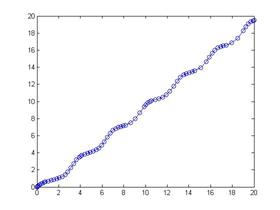
Необходимо реализовать метод Рунге-Кутта 4 порядка и решить задачу Коши для предложенной системы дифференциальных уравнений:

В М-файле с именем pr 8. m пишем:

Потом в командном окне вызываем функцию ode 45:

Решение систем дифференциальных уравнений в MATLAB

Решение систем дифференциальных уравнений.

Для решения систем дифференциальных уравнений существует несколько встроенных процедур. Рассмотрим применение процедуры ode45. Как один из возможных форматов вызова, можно предложить такой: [t,r]=ode45(@DiffEquationFunction,[Tstart,Tfinish], StartVector). Отметим, что процедура ode45 может решить систему уравнений следующего вида: , где — есть векторная функция .

Рассмотрим пример, иллюстрирующий создание исходной функции DiffEquationFunction для вызова ее процедурой ode45. Пусть некоторая точка массы движется в гравитационном поле неподвижных точек с массами и (см. рис.). Уравнение сил в гравитационном поле точек и будет следующим: . Как видим, данное дифференциальное уравнение имеет второй порядок. Но его можно свести к системе дифференциальных уравнений первого порядка: .

Будем считать, что данная задача является «плоской» и введем следующие обозначения: , , и . Исходя из таких обозначений, систему дифференциальных уравнений движения точки в гравитационном поле можно представить следующим образом: .

Без ущерба для сути решения, значение гравитационной постоянной примем равной 1, , , , .

В таком виде систему уравнений можно уже записать как файл-функцию, что мы и сделали, назвав ее threepoint(t,x).

M1=50; M2=0; C1x=5; C1y=0; C2x=0; C2y=10;

Решим систему дифференциальных уравнений, вызвав процедуру ode45 из файла-функции dynpoint.m.

x1=5; y1=0; x2=0; y2=10;

При таких начальных параметрах ( ) наша точка движется в поле одного объекта.

То, что мы получили вполне можно назвать приемлемым результатом. Нашей целью являлась корректная подготовка системы дифференциальных уравнений для ее решения процедурой ode45. С другой стороны, применяя иные встроенные процедуры можно получить отличающиеся в корне результаты.

Попробуем немного поэкспериментировать и введем значение . Это должно внести возмущения в орбиту движущейся точки.

Крестиком и звездочкой на графике отмечены соответственно и . Помимо процедуры ode45 существует еще ряд встроенных процедур решения систем дифференциальных уравнений. Их описание можно найти в книгах, указанных в списке литературы. Поскольку, решение систем дифференциальных уравнений является очень важным моментом, то мы не ограничимся одним примером.

Рассмотрим следующую задачу, опять же из физики. Рассмотрим траекторию движения пули под действием силы тяжести. При отсутствии сопротивления воздуха, как известно из курса средней школы, это будет парабола. Мы же рассмотрим случай, когда сила сопротивления воздуха пропорциональна квадрату скорости и противоположна направлению движения. Как говорит школьный курс физики, уравнение баланса сил будет следующим: . Учитывая то, что ускорение – производная скорости по времени, распишем это уравнение в векторном виде: . Где — плотность воздуха, — масса пули, — площадь поперечного сечения. Распишем это уравнение покоординатно: . В таком виде система дифференциальных уравнений готова для того, чтобы попытаться решить ее при помощи процедуры ode45. Пусть масса пули – 10 грамм, поперечник – 1 см 2 , плотность воздуха – 1 кг/м 3 . С такими данными мы составим файл-функцию airpoint.m.

g=10; ro=1; s=0.0001; m=0.01; k=ro*s/(2*m);

В такой системе уравнений аргументом являются скорость и время. Если мы хотим найти траекторию движения, то мы должны принять во внимание: . Полученные массивы точек , , можно в дальнейшем обработать. Произвести интерполяцию, аппроксимацию и т.д. Но мы интегрирование заменим суммированием: . В этом случае начальный момент времени равен 0, пуля находится в начале координат. Создадим файл-функцию dynairpoint, в которой вызовем процедуру ode45. В начальный момент времени скорость пули по горизонтали 800, по вертикали – 100.

Ode45 matlab система дифференциальных уравнений

Solve initial value problems for ordinary differential equations (ODEs)

where solver is one of ode45 , ode23 , ode113 , ode15s , ode23s , ode23t , or ode23tb .

odefun	A function that evaluates the right-hand side of the differential equations. All solvers solve systems of equations in the form or problems that involve a mass matrix, . The ode23s solver can solve only equations with constant mass matrices. ode15s and ode23t can solve problems with a mass matrix that is singular, i.e., differential-algebraic equations (DAEs).
tspan	A vector specifying the interval of integration, [t0,tf] . To obtain solutions at specific times (all increasing or all decreasing), use tspan = [t0,t1. tf] .
y0	A vector of initial conditions.
options	Optional integration argument created using the odeset function. See odeset for details.
p1,p2.	Optional parameters that the solver passes to odefun and all the functions specified in options ..

[T,Y] = solver (odefun,tspan,y0) with tspan = [t0 tf] integrates the system of differential equations from time t0 to tf with initial conditions y0 . Function f = odefun(t,y) , for a scalar t and a column vector y , must return a column vector f corresponding to . Each row in the solution array Y corresponds to a time returned in column vector T . To obtain solutions at the specific times t0 , t1. tf (all increasing or all decreasing), use tspan = [t0,t1. tf] .

[T,Y] = solver (odefun,tspan,y0,options) solves as above with default integration parameters replaced by property values specified in options , an argument created with the odeset function. Commonly used properties include a scalar relative error tolerance RelTol ( 1e-3 by default) and a vector of absolute error tolerances AbsTol (all componen t s are 1e-6 by default). See odeset for details.

[T,Y] = solver (odefun,tspan,y0,options,p1,p2. ) solves as above, passing the additional parameters p1,p2. to the function odefun , whenever it is called. Use options = [] as a place holder if no options are set.

[T,Y,TE,YE,IE] = solver (odefun,tspan,y0,options) solves as above while also finding where functions of , called event functions, are zero. For each event function, you specify whether the integration is to terminate at a zero and whether the direction of the zero crossing matters. Do this by setting the ‘Events’ property to a function, e.g., events or @events , and creating a function [ value , isterminal , direction ] = events ( t , y ). For the i th event function in events :

• value(i) is the value of the function.
• isterminal(i) = 1 if the integration is to terminate at a zero of this event function and 0 otherwise.
• direction(i) = 0 if all zeros are to be computed (the default), +1 if only the zeros where the event function increases, and -1 if only the zeros where the event function decreases.

Corresponding entries in TE , YE , and IE return, respectively, the time at which an event occurs, the solution at the time of the event, and the index i of the event function that vanishes.

sol = solver (odefun,[t0 tf],y0. ) returns a structure that you can use with deval to evaluate the solution at any point on the interval [t0,tf] . You must pass odefun as a function handle. The structure sol always includes these fields:

If you specify the Events option and events are detected, sol also includes these fields:

If you specify an output function as the value of the OutputFcn property, the solver calls it with the computed solution after each time step. Four output functions are provided: odeplot , odephas2 , odephas3 , odeprint . When you call the solver with no output arguments, it calls the default odeplot to plot the solution as it is computed. odephas2 and odephas3 produce two- and three-dimnesional phase plane plots, respectively. odeprint displays the solution components on the screen. By default, the ODE solver passes all components of the solution to the output function. You can pass only specific components by providing a vector of indices as the value of the OutputSel property. For example, if you call the solver with no output arguments and set the value of OutputSel to [1,3] , the solver plots solution components 1 and 3 as they are computed.

For the stiff solvers ode15s , ode23s , ode23t , and ode23tb , the Jacobian matrix is critical to reliability and efficiency. Use odeset to set Jacobian to @FJAC if FJAC(T,Y) returns the Jacobian or to the matrix if the Jacobian is constant. If the Jacobian property is not set (the default), is approximated by finite differences. Set the Vectorized property ‘ on ‘ if the ODE function is coded so that odefun ( T ,[ Y1,Y2 . ]) returns [ odefun ( T , Y1 ) ,odefun ( T , Y2 ) . ]. If is a sparse matrix, set the JPattern property to the sparsity pattern of , i.e., a sparse matrix S with S(i,j) = 1 if the i th component of depends on the j th component of , and 0 otherwise.

The solvers of the ODE suite can solve problems of the form , with time- and state-dependent mass matrix . (The ode23s solver can solve only equations with constant mass matrices.) If a problem has a mass matrix, create a function M = MASS(t,y) that returns the value of the mass matrix, and use odeset to set the Mass property to @MASS . If the mass matrix is constant, the matrix should be used as the value of the Mass property. Problems with state-dependent mass matrices are more difficult:

• If the mass matrix does not depend on the state variable and the function MASS is to be called with one input argument, t , set the MStateDependence property to ‘ none ‘.
• If the mass matrix depends weakly on , set MStateDependence to ‘ weak ‘ (the default) and otherwise, to ‘ strong ‘. In either case, the function MASS is called with the two arguments ( t , y ).

If there are many differential equations, it is important to exploit sparsity:

• Return a sparse .
• Supply the sparsity pattern of using the JPattern property or a sparse using the Jacobian property.
• For strongly state-dependent , set MvPattern to a sparse matrix S with S(i,j) = 1 if for any k , the ( i,k ) component of depends on component j of , and 0 otherwise.

If the mass matrix is singular, then is a differential algebraic equation. DAEs have solutions only when is consistent, that is, if there is a vector such that

. The ode15s and ode23t solvers can solve DAEs of index 1 provided that y0 is sufficiently close to being consistent. If there is a mass matrix, you can use odeset to set the MassSingular property to ‘yes’ , ‘no’ , or ‘maybe’ . The default value of ‘maybe’ causes the solver to test whether the problem is a DAE. You can provide yp0 as the value of the InitialSlope property. The default is the zero vector. If a problem is a DAE, and y0 and yp0 are not consistent, the solver treats them as guesses, attempts to compute consistent values that are close to the guesses, and continues to solve the problem. When solving DAEs, it is very advantageous to formulate the problem so that is a diagonal matrix (a semi-explicit DAE).

The algorithms used in the ODE solvers vary according to order of accuracy [6] and the type of systems (stiff or nonstiff) they are designed to solve. See Algorithms for more details.

Different solvers accept different parameters in the options list. For more information, see odeset and Improving ODE Solver Performance in the «Mathematics» section of the MATLAB documentation.

Parameters	ode45	ode23	ode113	ode15s	ode23s	ode23t	ode23tb
RelTol , AbsTol, NormControl
OutputFcn , OutputSel , Refine , Stats
Events
MaxStep , InitialStep
Jacobian, JPattern, Vectorized	—	—	—
Mass MStateDependence MvPattern MassSingular	— —	— —	— —		— — —		—
InitialSlope	—	—	—		—		—
MaxOrder , BDF	—	—	—		—	—	—

Example 1. An example of a nonstiff system is the system of equations describing the motion of a rigid body without external forces.

To simulate this system, create a function rigid containing the equations

In this example we change the error tolerances using the odeset command and solve on a time interval [0 12] with an initial condition vector [0 1 1] at time 0 .

Plotting the columns of the returned array Y versus T shows the solution

Example 2. An example of a stiff system is provided by the van der Pol equations in relaxation oscillation. The limit cycle has portions where the solution components change slowly and the problem is quite stiff, alternating with regions of very sharp change where it is not stiff.

To simulate this system, create a function vdp1000 containing the equations

For this problem, we will use the default relative and absolute tolerances ( 1e-3 and 1e-6 , respectively) and solve on a time interval of [0 3000] with initial condition vector [2 0] at time 0 .

Plotting the first column of the returned matrix Y versus T shows the solution

ode45 is based on an explicit Runge-Kutta (4,5) formula, the Dormand-Prince pair. It is a one-step solver — in computing y(t _n ) , it needs only the solution at the immediately preceding time point, y(t _n-1 ) . In general, ode45 is the best function to apply as a «first try» for most problems. [3]

ode23 is an implementation of an explicit Runge-Kutta (2,3) pair of Bogacki and Shampine. It may be more efficient than ode45 at crude tolerances and in the presence of moderate stiffness. Like ode45 , ode23 is a one-step solver. [2]

ode113 is a variable order Adams-Bashforth-Moulton PECE solver. It may be more efficient than ode45 at stringent tolerances and when the ODE file function is particularly expensive to evaluate. ode113 is a multistep solver — it normally needs the solutions at several preceding time points to compute the current solution. [7]

The above algorithms are intended to solve nonstiff systems. If they appear to be unduly slow, try using one of the stiff solvers below.

ode15s is a variable order solver based on the numerical differentiation formulas (NDFs). Optionally, it uses the backward differentiation formulas (BDFs, also known as Gear’s method) that are usually less efficient. Like ode113 , ode15s is a multistep solver. Try ode15s when ode45 fails, or is very inefficient, and you suspect that the problem is stiff, or when solving a differential-algebraic problem. [9], [10]

ode23s is based on a modified Rosenbrock formula of order 2. Because it is a one-step solver, it may be more efficient than ode15s at crude tolerances. It can solve some kinds of stiff problems for which ode15s is not effective. [9]

ode23t is an implementation of the trapezoidal rule using a «free» interpolant. Use this solver if the problem is only moderately stiff and you need a solution without numerical damping. ode23t can solve DAEs. [10]

ode23tb is an implementation of TR-BDF2, an implicit Runge-Kutta formula with a first stage that is a trapezoidal rule step and a second stage that is a backward differentiation formula of order two. By construction, the same iteration matrix is used in evaluating both stages. Like ode23s , this solver may be more efficient than ode15s at crude tolerances. [8], [1]

[1] Bank, R. E., W. C. Coughran, Jr., W. Fichtner, E. Grosse, D. Rose, and R. Smith, «Transient Simulation of Silicon Devices and Circuits,» IEEE Trans. CAD, 4 (1985), pp 436-451.

[2] Bogacki, P. and L. F. Shampine, «A 3(2) pair of Runge-Kutta formulas,» Appl. Math. Letters, Vol. 2, 1989, pp 1-9.

[3] Dormand, J. R. and P. J. Prince, «A family of embedded Runge-Kutta formulae,» J. Comp. Appl. Math., Vol. 6, 1980, pp 19-26.

[4] Forsythe, G. , M. Malcolm, and C. Moler, Computer Methods for Mathematical Computations, Prentice-Hall, New Jersey, 1977.

[5] Kahaner, D. , C. Moler, and S. Nash, Numerical Methods and Software, Prentice-Hall, New Jersey, 1989.

[6] Shampine, L. F. , Numerical Solution of Ordinary Differential Equations, Chapman & Hall, New York, 1994.

[7] Shampine, L. F. and M. K. Gordon, Computer Solution of Ordinary Differential Equations: the Initial Value Problem, W. H. Freeman, San Francisco, 1975.

[8] Shampine, L. F. and M. E. Hosea, «Analysis and Implementation of TR-BDF2,» Applied Numerical Mathematics 20, 1996.

[9] Shampine, L. F. and M. W. Reichelt, » The MATLAB ODE Suite ,» SIAM Journal on Scientific Computing, Vol. 18, 1997, pp 1-22.